When a Firm Is on the Inelastic Segment of Its Demand Curve, It Can

ten.2 The Monopoly Model

Learning Objectives

1. Explain the relationship between price and marginal revenue when a firm faces a downward-sloping need curve.
2. Explicate the human relationship between marginal revenue and elasticity along a linear need bend.
3. Apply the marginal decision dominion to explain how a monopoly maximizes profit.

Analyzing choices is a more complex challenge for a monopoly firm than for a perfectly competitive firm. After all, a competitive firm takes the market place price equally given and determines its profit-maximizing output. Considering a monopoly has its market all to itself, it can decide non only its output but its price as well. What kinds of price and output choices will such a business firm make?

We will answer that question in the context of the marginal decision dominion: a firm volition produce additional units of a good until marginal acquirement equals marginal cost. To apply that rule to a monopoly firm, we must get-go investigate the special relationship between demand and marginal revenue for a monopoly.

Monopoly and Marketplace Need

Because a monopoly firm has its market all to itself, it faces the marketplace need curve. Figure 10.3 "Perfect Competition Versus Monopoly" compares the demand situations faced past a monopoly and a perfectly competitive firm. In Panel (a), the equilibrium price for a perfectly competitive firm is determined by the intersection of the need and supply curves. The market supply curve is found simply by summing the supply curves of individual firms. Those, in plough, consist of the portions of marginal price curves that lie above the boilerplate variable cost curves. The marginal cost bend, MC, for a unmarried firm is illustrated. Detect the break in the horizontal axis indicating that the quantity produced by a single firm is a trivially small fraction of the whole. In the perfectly competitive model, one house has nothing to do with the determination of the market price. Each house in a perfectly competitive industry faces a horizontal demand bend defined by the market price.

Figure 10.three Perfect Contest Versus Monopoly

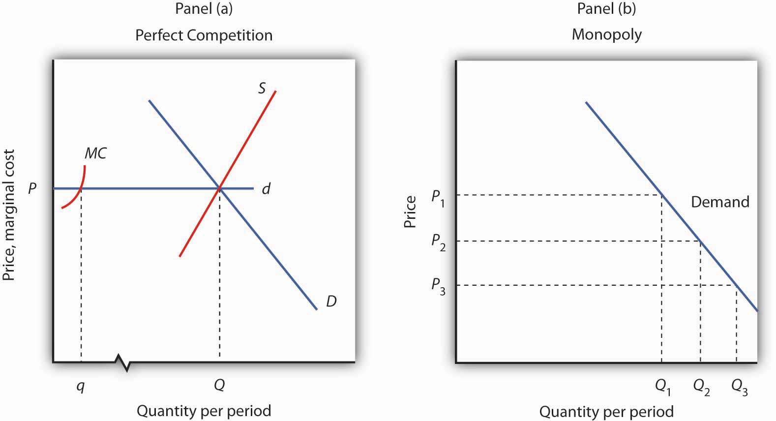
Panel (a) shows the determination of equilibrium price and output in a perfectly competitive market place. A typical firm with marginal cost bend MC is a price taker, choosing to produce quantity q at the equilibrium price P. In Console (b) a monopoly faces a down-sloping market demand curve. As a turn a profit maximizer, it determines its profit-maximizing output. Once it determines that quantity, however, the price at which information technology tin can sell that output is plant from the demand curve. The monopoly firm tin can sell boosted units only by lowering price. The perfectly competitive firm, by contrast, can sell whatever quantity it wants at the market price.

Contrast the state of affairs shown in Panel (a) with the one faced by the monopoly firm in Console (b). Considering it is the just supplier in the industry, the monopolist faces the down-sloping market place demand curve lonely. It may choose to produce any quantity. Simply, unlike the perfectly competitive house, which can sell all it wants at the going market price, a monopolist tin can sell a greater quantity but by cutting its price.

Suppose, for example, that a monopoly house can sell quantity Q ₁ units at a toll P ₁ in Panel (b). If it wants to increase its output to Q _two units—and sell that quantity—it must reduce its cost to P ₂. To sell quantity Q _iii it would have to reduce the price to P ₃. The monopoly firm may cull its price and output, but it is restricted to a combination of price and output that lies on the need curve. It could not, for example, accuse price P ₁ and sell quantity Q _iii. To be a price setter, a firm must face up a downward-sloping need bend.

Total Revenue and Price Elasticity

A firm'due south elasticity of demand with respect to price has of import implications for assessing the impact of a price alter on full acquirement. Also, the price elasticity of demand tin be different at different points on a firm'south demand bend. In this section, we shall see why a monopoly firm will always select a price in the elastic region of its demand bend.

Suppose the demand bend facing a monopoly firm is given by Equation 10.ane, where Q is the quantity demanded per unit of measurement of fourth dimension and P is the cost per unit:

Equation ten.one

[latex]Q = 10 - P[/latex]

This demand equation implies the demand schedule shown in Figure 10.4 "Need, Elasticity, and Total Revenue". Total acquirement for each quantity equals the quantity times the price at which that quantity is demanded. The monopoly firm's total revenue bend is given in Panel (b). Because a monopolist must cutting the price of every unit of measurement in order to increase sales, total revenue does non ever increase as output rises. In this case, total revenue reaches a maximum of $25 when v units are sold. Beyond 5 units, total revenue begins to decline.

Figure 10.4 Demand, Elasticity, and Total Revenue

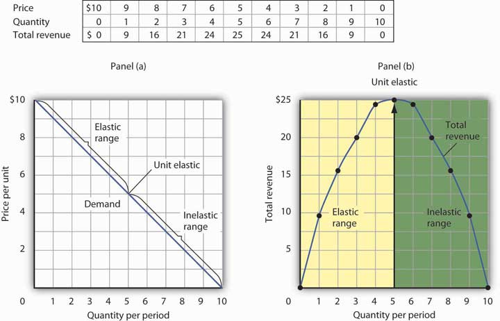
Suppose a monopolist faces the downwards-sloping need curve shown in Panel (a). In order to increase the quantity sold, it must cut the price. Full revenue is found past multiplying the price and quantity sold at each price. Total revenue, plotted in Console (b), is maximized at $25, when the quantity sold is v units and the price is $v. At that point on the demand curve, the cost elasticity of demand equals −i.

The demand curve in Console (a) of Figure 10.four "Demand, Elasticity, and Total Acquirement" shows ranges of values of the price elasticity of need. We have learned that price elasticity varies along a linear demand bend in a special style: Demand is price elastic at points in the upper half of the demand curve and price inelastic in the lower one-half of the need bend. If demand is price elastic, a cost reduction increases total revenue. To sell an additional unit, a monopoly firm must lower its price. The sale of one more unit of measurement will increment revenue considering the pct increase in the quantity demanded exceeds the per centum decrease in the price. The rubberband range of the demand bend corresponds to the range over which the total revenue curve is rise in Panel (b) of Effigy 10.4 "Demand, Elasticity, and Total Revenue".

If demand is price inelastic, a price reduction reduces full revenue because the percent increase in the quantity demanded is less than the percentage decrease in the price. Total revenue falls as the business firm sells additional units over the inelastic range of the need curve. The downwards-sloping portion of the full revenue bend in Panel (b) corresponds to the inelastic range of the demand bend.

Finally, call up that the midpoint of a linear demand curve is the point at which demand becomes unit toll elastic. That point on the total acquirement curve in Console (b) corresponds to the point at which total revenue reaches a maximum.

The relationship among price elasticity, demand, and total revenue has an of import implication for the selection of the turn a profit-maximizing price and output: A monopoly house will never choose a price and output in the inelastic range of the demand curve. Suppose, for example, that the monopoly business firm represented in Figure x.4 "Demand, Elasticity, and Full Revenue" is charging $iii and selling 7 units. Its total revenue is thus $21. Because this combination is in the inelastic portion of the demand curve, the firm could increase its full acquirement by raising its price. Information technology could, at the same fourth dimension, reduce its full cost. Raising price ways reducing output; a reduction in output would reduce total cost. If the house is operating in the inelastic range of its demand curve, then it is not maximizing profits. The business firm could earn a college profit past raising price and reducing output. Information technology will keep to raise its price until it is in the elastic portion of its demand curve. A profit-maximizing monopoly firm volition therefore select a price and output combination in the rubberband range of its demand bend.

Of course, the business firm could choose a betoken at which demand is unit of measurement price elastic. At that indicate, full revenue is maximized. But the house seeks to maximize profit, non total revenue. A solution that maximizes full acquirement will non maximize profit unless marginal cost is zero.

Demand and Marginal Revenue

In the perfectly competitive case, the additional acquirement a firm gains from selling an additional unit—its marginal revenue—is equal to the marketplace toll. The house'south need curve, which is a horizontal line at the market price, is besides its marginal revenue bend. But a monopoly firm tin sell an additional unit of measurement only past lowering the price. That fact complicates the human relationship between the monopoly's demand curve and its marginal revenue.

Suppose the firm in Figure 10.4 "Need, Elasticity, and Total Revenue" sells 2 units at a toll of $8 per unit. Its total revenue is $sixteen. Now it wants to sell a third unit of measurement and wants to know the marginal revenue of that unit. To sell 3 units rather than 2, the business firm must lower its toll to $7 per unit. Total revenue rises to $21. The marginal revenue of the third unit is thus $5. But the cost at which the firm sells 3 units is $7. Marginal revenue is less than toll.

To run across why the marginal acquirement of the third unit is less than its toll, nosotros need to examine more carefully how the sale of that unit of measurement affects the business firm'southward revenues. The firm brings in $7 from the sale of the third unit. Simply selling the third unit of measurement required the firm to charge a price of $vii instead of the $eight the firm was charging for 2 units. Now the firm receives less for the first 2 units. The marginal acquirement of the tertiary unit of measurement is the $seven the firm receives for that unit minus the $one reduction in revenue for each of the kickoff 2 units. The marginal acquirement of the third unit is thus $5. (In this affiliate nosotros presume that the monopoly firm sells all units of output at the aforementioned price. In the adjacent affiliate, nosotros volition look at cases in which firms charge unlike prices to different customers.)

Marginal acquirement is less than price for the monopoly firm. Effigy x.5 "Demand and Marginal Acquirement" shows the relationship between demand and marginal revenue, based on the need curve introduced in Effigy 10.iv "Need, Elasticity, and Total Revenue". As always, nosotros follow the convention of plotting marginal values at the midpoints of the intervals.

Figure 10.v Demand and Marginal Revenue

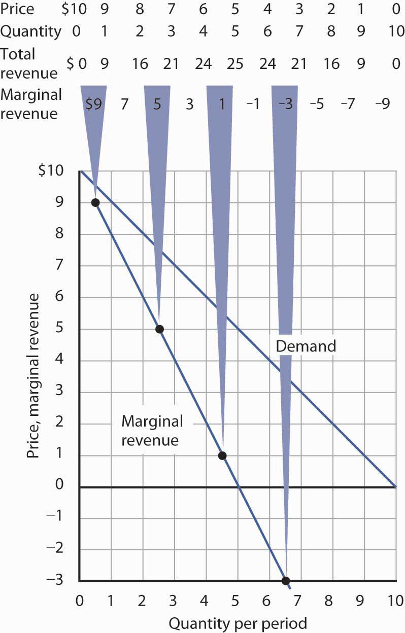
The marginal acquirement curve for the monopoly firm lies below its demand curve. It shows the additional acquirement gained from selling an boosted unit. Notice that, every bit e'er, marginal values are plotted at the midpoints of the corresponding intervals.

When the need bend is linear, as in Effigy 10.5 "Demand and Marginal Revenue", the marginal acquirement bend can be placed according to the following rules: the marginal revenue curve is ever below the demand curve and the marginal revenue curve will bisect whatever horizontal line drawn between the vertical axis and the demand curve. To put it some other way, the marginal acquirement curve will be twice as steep as the need curve. The demand curve in Figure 10.5 "Demand and Marginal Revenue" is given by the equation Q=10−P, which can be written P=10−Q. The marginal acquirement bend is given by P=x−2Q, which is twice every bit steep as the need curve.

The marginal revenue and demand curves in Figure ten.five "Demand and Marginal Revenue" follow these rules. The marginal acquirement curve lies below the demand curve, and it bisects any horizontal line drawn from the vertical axis to the demand curve. At a price of $six, for example, the quantity demanded is 4. The marginal acquirement bend passes through 2 units at this price. At a toll of 0, the quantity demanded is 10; the marginal revenue curve passes through 5 units at this point.

Just as at that place is a human relationship betwixt the business firm'due south need curve and the cost elasticity of need, there is a relationship between its marginal revenue curve and elasticity. Where marginal acquirement is positive, demand is price elastic. Where marginal revenue is negative, demand is price inelastic. Where marginal revenue is zip, demand is unit of measurement price elastic.

When marginal acquirement is …	then need is …
positive,	price elastic.
negative,	cost inelastic.
zero,	unit price rubberband.

A firm would non produce an additional unit of output with negative marginal acquirement. And, bold that the production of an additional unit has some cost, a firm would not produce the extra unit if it has zero marginal revenue. Considering a monopoly firm will generally operate where marginal acquirement is positive, we see once once again that it will operate in the elastic range of its demand bend.

Monopoly Equilibrium: Applying the Marginal Decision Rule

Profit-maximizing beliefs is ever based on the marginal conclusion rule: Additional units of a good should be produced equally long as the marginal acquirement of an additional unit exceeds the marginal toll. The maximizing solution occurs where marginal revenue equals marginal cost. As always, firms seek to maximize economic profit, and costs are measured in the economic sense of opportunity cost.

Effigy 10.6 "The Monopoly Solution" shows a demand curve and an associated marginal acquirement curve facing a monopoly business firm. The marginal cost curve is like those we derived earlier; information technology falls over the range of output in which the firm experiences increasing marginal returns, and so rises as the firm experiences diminishing marginal returns.

Figure ten.vi The Monopoly Solution

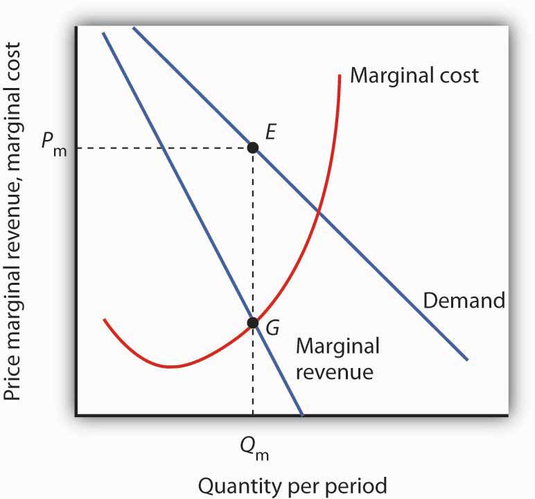
The monopoly house maximizes profit past producing an output Q _yard at point G, where the marginal revenue and marginal toll curves intersect. It sells this output at cost P _m.

To make up one's mind the profit-maximizing output, we notation the quantity at which the firm'due south marginal acquirement and marginal cost curves intersect (Q _m in Figure 10.6 "The Monopoly Solution"). We read up from Q _{one thousand} to the demand curve to find the cost P _chiliad at which the firm can sell Q _m units per period. The turn a profit-maximizing price and output are given by point E on the demand bend.

Thus we can determine a monopoly firm'south profit-maximizing price and output past following three steps:

1. Determine the demand, marginal revenue, and marginal cost curves.
2. Select the output level at which the marginal acquirement and marginal toll curves intersect.
3. Decide from the need curve the price at which that output can be sold.

Figure 10.7 Computing Monopoly Profit

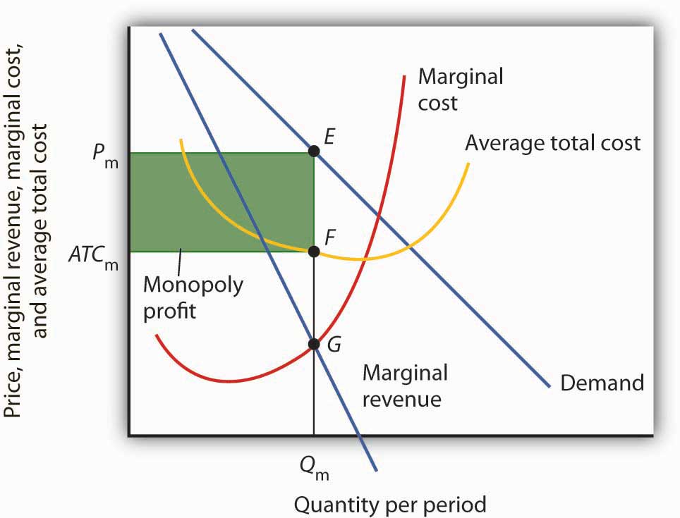
A monopoly firm's turn a profit per unit of measurement is the difference between price and boilerplate full cost. Total profit equals profit per unit times the quantity produced. Full profit is given by the area of the shaded rectangle ATC _thousand P _mEF.

Once we accept determined the monopoly firm's price and output, we can make up one's mind its economic profit past calculation the firm's average total cost bend to the graph showing demand, marginal revenue, and marginal cost, as shown in Figure 10.vii "Computing Monopoly Profit". The average total price (ATC) at an output of Q _thou units is ATC _k. The firm's profit per unit of measurement is thus P _m – ATC _{one thousand}. Total profit is plant past multiplying the firm's output, Q _g, past turn a profit per unit of measurement, so total turn a profit equals Q _m(P _m – ATC _m)—the area of the shaded rectangle in Figure 10.7 "Computing Monopoly Turn a profit".

Heads Up!

Dispelling Myths Well-nigh Monopoly

Three common misconceptions about monopoly are:

1. Because there are no rivals selling the products of monopoly firms, they tin can charge whatsoever they desire.
2. Monopolists will accuse whatever the market will bear.
3. Because monopoly firms have the marketplace to themselves, they are guaranteed huge profits.

As Figure 10.vi "The Monopoly Solution" shows, once the monopoly firm decides on the number of units of output that will maximize profit, the price at which it can sell that many units is constitute past "reading off" the demand curve the cost associated with that many units. If it tries to sell Q _{one thousand} units of output for more P _m, some of its output volition go unsold. The monopoly business firm tin set its price, but is restricted to price and output combinations that lie on its demand curve. It cannot just "charge any it wants." And if it charges "all the market will bear," information technology will sell either 0 or, at virtually, 1 unit of measurement of output.

Neither is the monopoly house guaranteed a profit. Consider Figure 10.vii "Computing Monopoly Profit". Suppose the average total cost bend, instead of lying below the need bend for some output levels every bit shown, were instead everywhere to a higher place the demand curve. In that case, the monopoly volition incur losses no matter what cost it chooses, since average total cost will always be greater than whatsoever toll it might charge. As is the case for perfect competition, the monopoly firm can continue producing in the curt run so long as price exceeds boilerplate variable price. In the long run, information technology volition stay in concern only if information technology tin can cover all of its costs.

Primal Takeaways

• If a firm faces a downward-sloping demand curve, marginal revenue is less than price.
• Marginal revenue is positive in the elastic range of a need bend, negative in the inelastic range, and zero where demand is unit of measurement price elastic.
• If a monopoly firm faces a linear demand curve, its marginal acquirement bend is too linear, lies below the demand curve, and bisects whatever horizontal line fatigued from the vertical axis to the demand curve.
• To maximize profit or minimize losses, a monopoly firm produces the quantity at which marginal cost equals marginal acquirement. Its cost is given by the point on the need curve that corresponds to this quantity.

Try It!

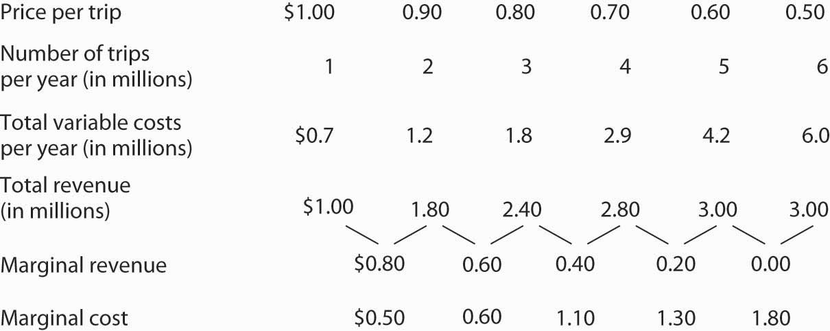
The Troll Road Company is considering building a toll road. Information technology estimates that its linear demand curve is as shown below. Assume that the stock-still cost of the road is $0.5 million per year. Maintenance costs, which are the merely other costs of the road, are likewise given in the tabular array.

Tolls per trip	$1.00	0.90	0.eighty	0.70	0.lx	0.50
Number of trips per year (in millions)	ane	2	three	4	5	vi
Maintenance cost per year (in millions)	$0.7	one.2	1.viii	ii.9	iv.ii	6.0

1. Using the midpoint convention, compute the profit-maximizing level of output.
2. Using the midpoint convention, what price volition the visitor accuse?
3. What is marginal acquirement at the profit-maximizing output level? How does marginal revenue compare to toll?

Instance in Signal: Turn a profit-Maximizing Hockey Teams

Figure 10.eight

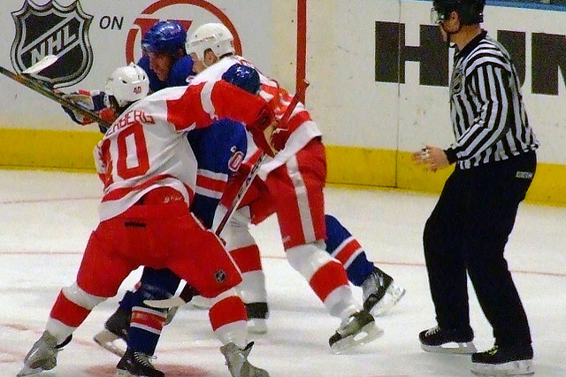
Duluoz cats – face off – CC Past-NC-ND 2.0.

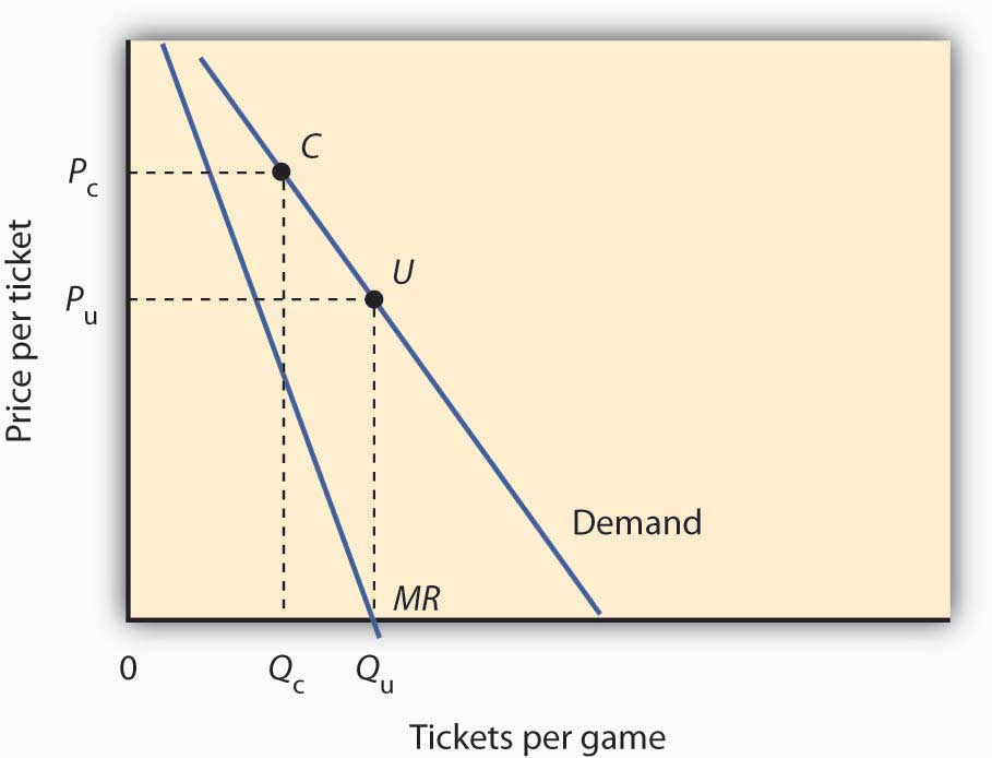
Honey of the game? Beloved of the city? Are those the factors that influence owners of professional sports teams in setting admissions prices? Four economists at the University of Vancouver accept what they think is the answer for one group of teams: professional person hockey teams gear up admission prices at levels that maximize their profits. They regard hockey teams as monopoly firms and utilise the monopoly model to examine the team's behavior.

The economists, Donald Chiliad. Ferguson, Kenneth Grand. Stewart, John Colin H. Jones, and Andre Le Dressay, used data from three seasons to estimate demand and marginal revenue curves facing each team in the National Hockey League. They found that demand for a squad'due south tickets is affected by population and income in the team'southward dwelling house city, the team's standing in the National Hockey League, and the number of superstars on the squad.

Because a sports team's costs do not vary significantly with the number of fans who attend a given game, the economists assumed that marginal toll is zero. The profit-maximizing number of seats sold per game is thus the quantity at which marginal revenue is zip, provided a team's stadium is large plenty to concord that quantity of fans. This unconstrained quantity is labeled Q _u, with a corresponding cost P _u in the graph.

Stadium size and the demand curve facing a team might preclude the team from selling the profit-maximizing quantity of tickets. If its stadium holds only Q _c fans, for example, the squad will sell that many tickets at price P _c; its marginal acquirement is positive at that quantity. Economic theory thus predicts that the marginal acquirement for teams that consistently sell out their games will be positive, and the marginal revenue for other teams will be zero.

The economists' statistical results were consistent with the theory. They found that teams that don't typically sell out their games operate at a quantity at which marginal revenue is about null, and that teams with sellouts have positive marginal revenue. "Information technology'due south articulate that these teams are very sophisticated in their use of pricing to maximize profits," Mr. Ferguson said.

Effigy 10.9

Sources: Donald G. Ferguson et al., "The Pricing of Sports Events: Do Teams Maximize Profit?" Journal of Industrial Economics 39(3) (March 1991): 297–310 and personal interview.

Answer to Try It! Problem

Maintenance costs institute the variable costs associated with building the route. In order to answer the showtime four parts of the question, you will demand to compute total revenue, marginal acquirement, and marginal cost, as shown at right:

1. Using the "midpoint" convention, the profit-maximizing level of output is 2.v million trips per yr. With that number of trips, marginal revenue ($0.60) equals marginal toll ($0.60).
2. Again, we utilize the "midpoint" convention. The visitor will charge a cost of $0.85.
3. The marginal revenue is $0.60, which is less than the $0.85 toll (price).

Figure 10.10

spencerthersenight.blogspot.com

Source: https://open.lib.umn.edu/principleseconomics/chapter/10-2-the-monopoly-model/

Share this post